Trajectory Optimization: DIRCOL and iLQR

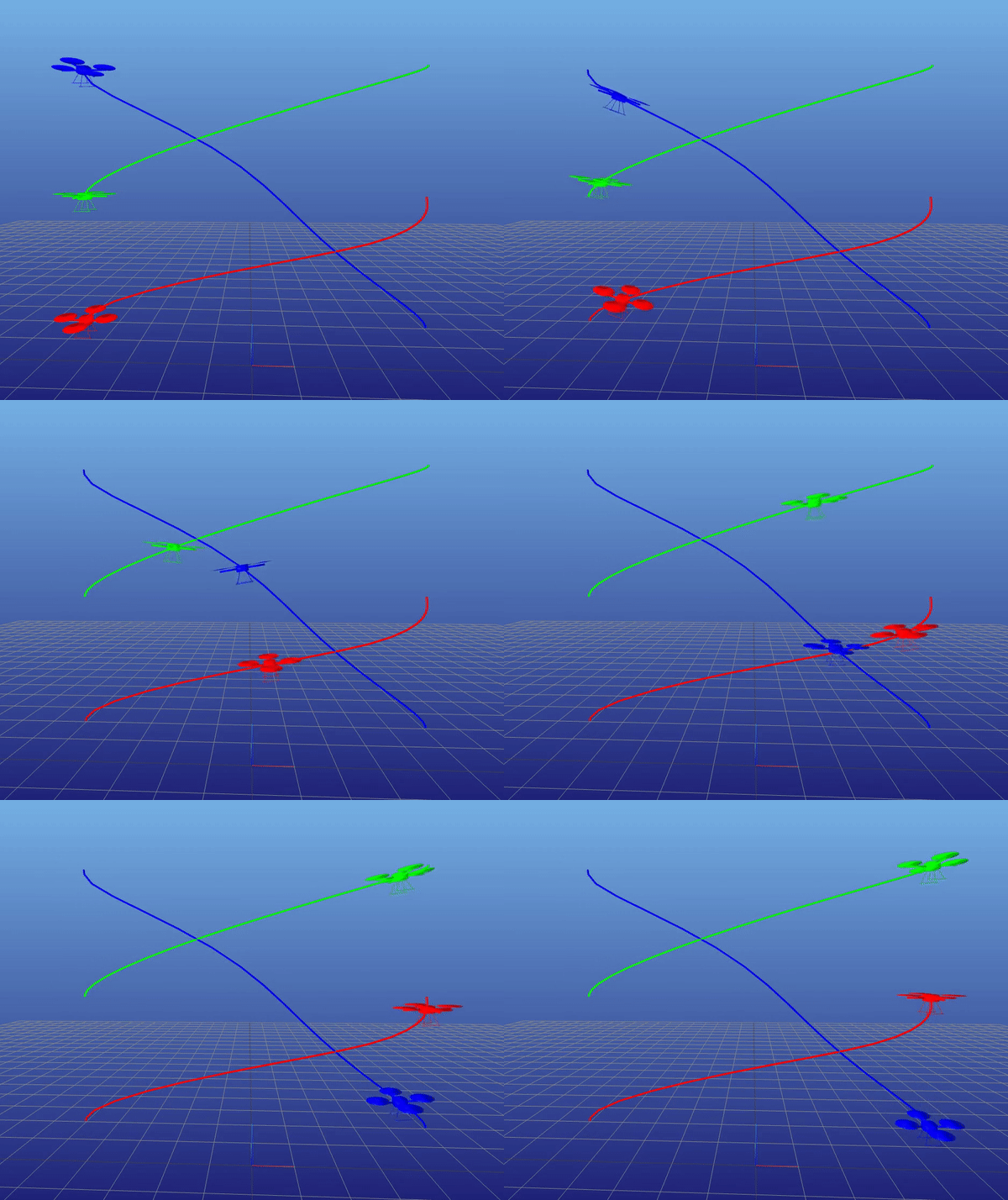
Project Overview

How do you compute the best path for a robot to follow? This project explores trajectory optimization—algorithms that find optimal motion plans by minimizing cost (like energy or time) while respecting physical constraints. I implemented two approaches: Direct Collocation (DIRCOL), which converts the problem into a large system of equations solved all at once, and iterative LQR (iLQR), which refines a trajectory through repeated local improvements. Both generate open-loop plans, which I then track using Time-Varying LQR (TVLQR) feedback control.

Systems and Methods

• Cart-pole swing-up — DIRCOL with Hermite-Simpson integration
• Quadrotor aerobatics — iLQR with RK4 discretization
• Multi-quadrotor — collision avoidance via inequality constraints
• TVLQR tracking — closed-loop control with model mismatch

DIRCOL for Cart-Pole

Direct Collocation transforms the continuous 'find the best trajectory' problem into a finite set of decision variables that standard optimization solvers can handle. Instead of solving differential equations directly, we represent the trajectory as a sequence of states and controls at discrete time points. Hermite-Simpson integration connects these points with smooth curves that approximate the true physics. The solver (IPOPT) then finds values that minimize cost while satisfying all constraints.

1# Stage cost: quadratic in state error and control
2for i = 1:(N-1)
3    J += 0.5 * (x[i] - xg)' * Q * (x[i] - xg)
4    J += 0.5 * u[i]' * R * u[i]
5end
6J += 0.5 * (x[N] - xg)' * Qf * (x[N] - xg)

Equality constraints enforce dynamics (via collocation) plus boundary conditions:

1constraints = [x[1] - x_ic;      # initial state
2               x[N] - x_goal;    # terminal state  
3               dynamics_residuals]  # Hermite-Simpson

Cart-Pole Swing-Up

The cart-pole is a classic control problem: balance a pole on a moving cart by pushing the cart left or right. The challenge is swinging the pole from hanging down to standing upright—a maneuver requiring carefully timed forces. Hermite-Simpson integration approximates the physics between time steps using cubic polynomials, giving much better accuracy than simple Euler steps:

1function hermite_simpson(p, x1, x2, u, dt)
2    xm = 0.5*(x1+x2) + (dt/8)*(f(x1,u) - f(x2,u))
3    return x1 + (dt/6)*(f(x1,u) + 4*f(xm,u) + f(x2,u)) - x2
4end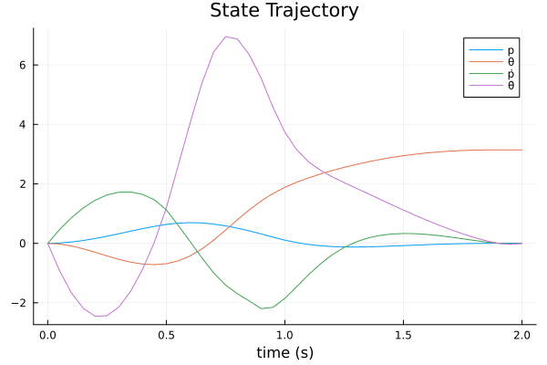

Cart-pole state trajectory from DIRCOL

TVLQR Tracking

The DIRCOL solution gives us an open-loop plan—a pre-computed sequence of controls. But real systems drift from the plan due to disturbances and modeling errors. TVLQR adds feedback: it computes correction gains at each time step that push the system back toward the planned trajectory. The controller applies both the planned control (feedforward) and error corrections (feedback). I simulate the closed-loop system using RK4 (Runge-Kutta 4th order), a standard numerical integration method:

1function rk4(p, x, u, dt)
2    k1 = dt * f(x, u)
3    k2 = dt * f(x + k1/2, u)
4    k3 = dt * f(x + k2/2, u)
5    k4 = dt * f(x + k3, u)
6    return x + (k1 + 2*k2 + 2*k3 + k4)/6
7end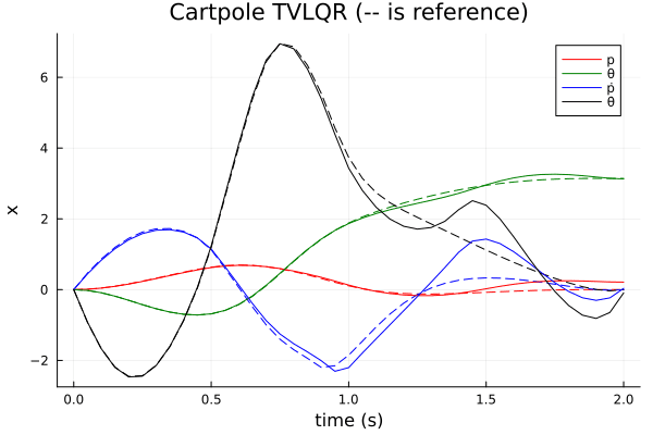

TVLQR tracking with model mismatch

iLQR for Quadrotor

While DIRCOL solves everything at once, iterative LQR (iLQR) takes a different approach: start with an initial guess trajectory, then repeatedly improve it. Each iteration approximates the nonlinear system as locally linear around the current trajectory, solves the simpler linear problem (standard LQR), then updates the trajectory. This process converges to a locally optimal solution. Here I apply it to a 6-DOF quadrotor performing aerobatic maneuvers.

Cost Expansion

iLQR needs to know how the cost changes as we adjust states and controls. We compute these gradients (first derivatives) and Hessians (second derivatives) using automatic differentiation—the computer calculates exact derivatives by tracking operations:

1Qxx = FD.hessian(dx -> stage_cost(dx, u, k), x)
2Qx  = FD.gradient(dx -> stage_cost(dx, u, k), x)
3Quu = FD.hessian(du -> stage_cost(x, du, k), u)
4Qu  = FD.gradient(du -> stage_cost(x, du, k), u)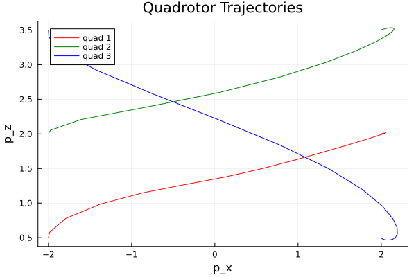

Quadrotor aerobatic trajectory via iLQR

Quadrotor Tracking

Just like with the cart-pole, the iLQR trajectory is open-loop and needs feedback for robustness. I apply TVLQR to track the aerobatic maneuver, testing with intentional parameter mismatches (e.g., wrong mass estimates) to verify the controller corrects for modeling errors.

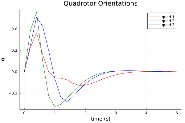
Quadrotor orientation during TVLQR tracking

Multi-Quadrotor Collision Avoidance

The final challenge: coordinate three quadrotors swapping positions without crashing into each other. I extend DIRCOL with inequality constraints that require each pair of quadrotors to stay at least a minimum distance apart at every time step. The optimizer finds trajectories that complete the reorientation while respecting these safety margins:

1# Distance constraints (squared to avoid sqrt)
2for i = 1:N-1
3    px1, px2, px3 = x[i][1:2], x[i][7:8], x[i][13:14]
4    c[i*3-2] = norm(px1-px2)^2 - d_min^2  # >= 0
5    c[i*3-1] = norm(px2-px3)^2 - d_min^2
6    c[i*3]   = norm(px1-px3)^2 - d_min^2
7end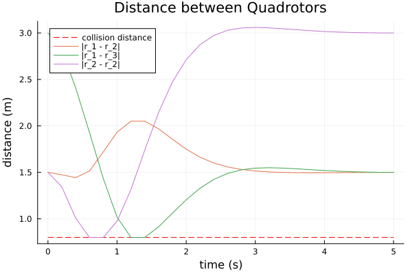

Inter-quadrotor distances during maneuver

Three quadrotors reorienting with collision avoidance

Conclusion

This project built up a toolkit for robot motion planning, from computing optimal trajectories to tracking them reliably:

• DIRCOL converts continuous motion planning into a solvable optimization problem
• iLQR finds optimal trajectories through iterative refinement
• TVLQR adds feedback control for robust real-world tracking
• Inequality constraints enforce safety requirements like collision avoidance