Iterative Learning and Hybrid Control

Project Overview

Some problems are best solved by practice: try something, see what went wrong, adjust, and try again. Iterative Learning Control (ILC) formalizes this intuition—the controller learns from each attempt to do better next time. Meanwhile, hybrid systems have dynamics that suddenly change (like a foot hitting the ground while walking). This project tackles both: ILC for a car's evasive maneuver, and hybrid trajectory optimization for bipedal walking.

Topics Explored

• Iterative Learning Control — refine trajectories by learning from previous runs
• Hybrid dynamics — handle discrete mode switches (foot strikes)
• Bipedal walking — optimize gait with contact constraints
• Nonlinear bicycle model — realistic car dynamics

Iterative Learning Control for Car Maneuver

Picture a driver practicing a 'moose test'—that sudden swerve to avoid an obstacle. Each run, they get a little better. ILC does the same thing mathematically: simulate the car, compare to the desired path, compute corrections, and repeat. After a few iterations, the controller has learned to nail the maneuver.

Bicycle Model Dynamics

We model the car using a nonlinear bicycle model—a simplification that captures steering and velocity dynamics without modeling each wheel individually:

1function car_dynamics(model, x, u)
2    px, py, θ, δ, v = x  # position, heading, steering, velocity
3    a, δdot = u          # acceleration, steering rate
4    
5    β = atan(model.lr * δ, model.L)  # slip angle
6    xdot = [v*cos(θ+β), v*sin(θ+β),  # velocity components
7            v*cos(β)*tan(δ)/model.L,  # yaw rate
8            δdot, a]                   # steering/accel
9    return xdot
10end

ILC Update Step

Each iteration, we linearize around the current trajectory and solve a convex optimization to find control corrections that reduce tracking error:

1# ILC update: minimize tracking error via convex optimization
2ΔX, ΔU = cvx.Variable(nx, N), cvx.Variable(nu, N-1)
3cost = sum(quadform(X[k] + ΔX[:,k] - Xref[k], Q) for k=1:N)
4constraints = [ΔX[:,1] == 0]  # start from actual state
5for k = 1:N-1
6    constraints += ΔX[:,k+1] == A[k]*ΔX[:,k] + B[k]*ΔU[:,k]
7end
8solve!(minimize(cost), constraints)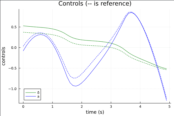

Car trajectory converging to reference over ILC iterations

Hybrid Trajectory Optimization for Bipedal Walking

Walking is fundamentally hybrid: smooth leg swings interrupted by sudden foot strikes. The physics changes instantly when a foot hits the ground—velocities reset, forces redistribute. Standard trajectory optimization assumes smooth dynamics, so we need special handling for these discrete jumps between modes.

Three-Mass Model

The biped is simplified to three point masses: one body, two feet. Each leg acts like a telescoping rod that can push but not pull. The dynamics switch depending on which foot is planted:

1# Stance dynamics depend on which foot is grounded
2if k in stance1_phase
3    xdot = stance1_dynamics(model, x, u)  # foot 1 planted
4elseif k in stance2_phase
5    xdot = stance2_dynamics(model, x, u)  # foot 2 planted
6end

Jump Maps (Foot Strikes)

When a swing foot hits the ground, it's an inelastic collision—the foot's velocity instantly goes to zero while other states continue. This discrete reset is the 'jump map':

1function jump1_map(x)
2    # Foot 1 hits ground: zero out its velocity
3    return [x[1:8]; 0.0; 0.0; x[11:12]]
4end

Trajectory Optimization

We use IPOPT to find a trajectory that tracks a reference gait while respecting hybrid dynamics. The optimizer enforces that stance foot velocity stays zero and leg lengths stay within bounds:

1# Dynamics constraints switch based on gait phase
2for k = 1:N-1
3    if k in M1 && !(k in J1)      # foot 1 stance
4        c[k] = x[k+1] - rk4(stance1_dynamics, x[k], u[k])
5    elseif k in J1                 # foot 1 strike
6        c[k] = x[k+1] - jump2_map(rk4(stance1_dynamics, ...))
7    end
8end

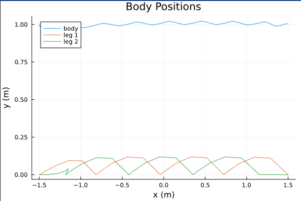
Body and foot trajectories during one gait cycle

Conclusion

This project explored two powerful ideas: learning from repetition and handling systems that suddenly change behavior. Both are essential for real-world robotics.

• ILC improves control by learning from each trial—no perfect model needed
• Hybrid dynamics capture the reality of contact: smooth motion interrupted by impacts
• Jump maps handle the instantaneous velocity resets at foot strikes
• Mode-dependent constraints let the optimizer know which foot is planted when

These techniques extend optimal control to messy real-world problems where models are imperfect and physics has discontinuities.