Optimal Control of Linear Systems

Project Overview

How do you make a robot move 'optimally'—minimizing energy, time, or error? Optimal control provides the math. This project implements several foundational techniques: LQR (Linear Quadratic Regulator) finds the best feedback controller for linear systems, TVLQR extends this to track time-varying trajectories, and MPC (Model Predictive Control) handles constraints by replanning in real-time.

Systems Studied

• Double integrator — position/velocity with acceleration control
• Cartpole — stabilization and swing-up trajectory tracking
• Spacecraft rendezvous — Clohessy-Wiltshire relative motion

Finite-Horizon LQR

Given a fixed time window, what's the best way to steer a system to a goal? Finite-Horizon LQR answers this by minimizing a 'cost' that penalizes both being far from the goal (state error) and using too much control effort. The math is elegant: the optimal solution is a linear feedback law, and we can compute it by solving either a convex optimization problem or a Riccati recursion (working backwards from the final time). I tested this on a simple double integrator (think: a mass you can push).

1cost = sum(quadform(X[:,k], Q) + quadform(U[:,k], R) for k=1:N-1)
2cost += quadform(X[:,N], Qf)  # terminal cost
3
4problem.constraints += X[:,1] == x_ic
5for k=1:N-1
6    problem.constraints += X[:,k+1] == A*X[:,k] + B*U[:,k]
7end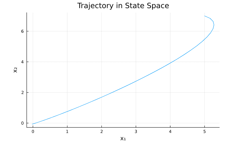

Double integrator trajectory using Finite-Horizon LQR

Bellman's Principle

Here's a beautiful insight: if you've found the optimal path from A to C (passing through B), then the portion from B to C is also optimal for that sub-problem. This is Bellman's Principle of Optimality—it's why dynamic programming works. I verified this experimentally: starting a new optimization from an intermediate state along the optimal trajectory gives the same remaining path.

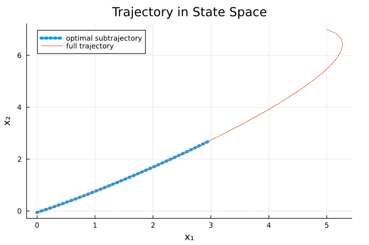
Trajectory comparison validating Bellman's Principle

Infinite-Horizon LQR

What if there's no fixed end time—you just want to stay at a goal forever? Infinite-Horizon LQR handles this by finding a single, constant feedback gain that works for all time. The math converges to a steady-state solution of the Riccati equation (called DARE). I used this to balance a cart-pole at its unstable upright position—the controller constantly corrects small deviations.

1for _ = 1:max_iters
2    K = (R + B'*P*B) \ (B'*P*A)
3    P_new = Q + K'*R*K + (A-B*K)'*P*(A-B*K)
4    norm(P_new - P) <= tol && return P_new, K
5    P = P_new
6end

Not every starting position can be stabilized—if the pole starts too far from upright, no controller can save it. The basin of attraction shows which initial conditions lead to success. I also tuned the cost matrices Q and R to keep control forces within realistic motor limits.

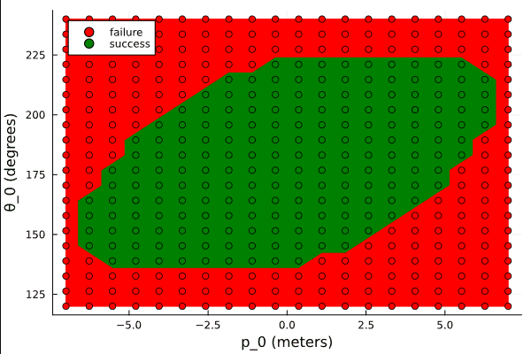
Basin of attraction for the cartpole LQR controller

Time-Varying LQR (TVLQR)

Regular LQR stabilizes around a single point. But what if you want to follow a moving reference—like a swing-up trajectory? Time-Varying LQR (TVLQR) computes different feedback gains for each moment in time by linearizing the system along the reference path. The controller combines the planned control (feedforward) with corrections for any deviations (feedback):

1for k = N-1:-1:1
2    K[k] = (R + B[k]'*P[k+1]*B[k]) \ (B[k]'*P[k+1]*A[k])
3    P[k] = Q + A[k]'*P[k+1]*(A[k] - B[k]*K[k])
4end
5# Control: u[k] = Uref[k] - K[k]*(x[k] - Xref[k])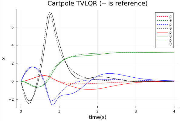

Cartpole swing-up tracking using TVLQR

Spacecraft Rendezvous

How does a spacecraft approach another in orbit? The Clohessy-Wiltshire equations describe relative motion between two orbiting objects—they're linear, making them perfect for LQR. The goal is to reach the target spacecraft while using minimal fuel (thrust).

• State — relative position and velocity (6D)
• Control — thrust accelerations in each axis
• Objective — reach target while minimizing fuel

Convex Trajectory Optimization

Real systems have limits: motors can only push so hard, spacecraft must avoid obstacles. Convex optimization lets us encode these as explicit constraints. The solver finds the best trajectory that respects all the rules—something basic LQR can't guarantee:

1problem.constraints += X[:,1] == x0
2problem.constraints += X[:,N] == xg
3for k=1:N-1
4    problem.constraints += U[:,k] >= u_min
5    problem.constraints += U[:,k] <= u_max
6end

Model Predictive Control (MPC)

What if conditions change? Model Predictive Control (MPC) replans at every timestep. It solves a finite-horizon optimization starting from wherever you currently are, applies only the first control action, then immediately replans with updated information. This 'receding horizon' approach handles disturbances and model errors gracefully—if something unexpected happens, you just replan:

1# At each timestep:
2problem.constraints += X_pred[:,1] == x_current
3solve!(problem)
4u_apply = U_pred.value[:,1]  # apply first control only

MPC Advantages

• Constraint satisfaction — bounds respected at each step
• Disturbance rejection — replanning corrects errors
• Receding horizon — computational tractability

Conclusion

This project built up from simple feedback control to sophisticated constrained optimization. The progression shows how each technique addresses different challenges:

• LQR — the foundation: optimal feedback for staying at a goal
• TVLQR — follow a planned trajectory with time-varying corrections
• MPC — handle constraints and adapt to real-time changes
• Convex optimization — the unifying framework that makes it all tractable