Robotic Arm Control and Trajectory Generation for Jenga

Project Introduction

How do you teach a robot arm to play Jenga? It needs to know where its hand is (forward kinematics), how to reach a target position (inverse kinematics), and how to move smoothly without knocking over the tower (trajectory planning). This capstone project tackled all three challenges for a 5-DOF articulated arm, implementing the math from scratch in MATLAB.

Conceptual DH Frame Assignment

Coordinate frames were assigned to each joint following the Denavit-Hartenberg convention: z-axis along the joint axis, x-axis normal to current and previous z-axes.

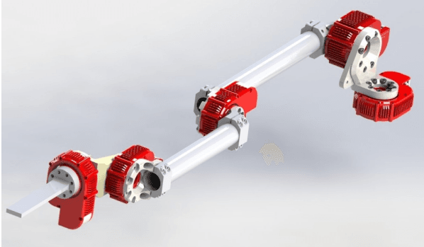
Robotic arm with Denavit-Hartenberg frame assignments.

DH Parameter Extraction

Before computing anything, we need a consistent way to describe the robot's geometry. Denavit-Hartenberg (DH) parameters are a standard convention: four numbers per joint that fully specify how each link connects to the next. We measured the physical arm and extracted these parameters—think of it as creating a mathematical blueprint of the robot.

Parameter Definitions

• a_i — link length (distance along x-axis)
• α_i — link twist (rotation about x-axis)
• d_i — link offset (distance along z-axis)
• θ_i — joint angle (rotation about z-axis)

1Link | a_i   | α_i   | d_i    | θ_i
2-----|-------|-------|--------|----------
31    | 0     | π/2   | 56.05  | variable
42    | 400   | 0     | 94     | variable
53    | 334   | -π/2  | 3      | variable
64    | 0     | π/2   | 39     | variable
75    | 0     | 0     | 108.05 | variable

Forward Kinematics

Given the joint angles, where is the gripper? Forward kinematics answers this by chaining together transformations from base to tip. Each joint adds a rotation and translation; multiply them all together and you get the end-effector's position and orientation. It's like following a series of 'turn left, go forward, rotate' instructions.

Transformation Convention

The transformation from frame i to frame i-1 follows the standard DH convention:

Expanding this yields the general transformation matrix:

1function H = Homog(theta, a, alpha, d)
2% Homogeneous transformation using DH params
3  H = [
4    cos(theta), -sin(theta)*cos(alpha), ...
5      sin(theta)*sin(alpha), a*cos(theta);
6    sin(theta),  cos(theta)*cos(alpha), ...
7     -cos(theta)*sin(alpha), a*sin(theta);
8    0,           sin(alpha), cos(alpha), d;
9    0,           0,          0,          1
10  ];
11end
12
13function T = forward_kinematics(dh, q)
14% Compute end-effector transformation
15% dh: [a, alpha, d, theta_offset] per row
16% q:  joint angles vector
17  T = eye(4);
18  for i = 1:size(dh, 1)
19    theta_i = q(i) + dh(i, 4);
20    H_i = Homog(theta_i, dh(i,1), ...
21                dh(i,2), dh(i,3));
22    T = T * H_i;
23  end
24end

Analytical Inverse Kinematics

The harder problem: given a target position for the gripper, what joint angles get us there? Inverse kinematics is like solving the forward problem backwards—and it's much trickier. There might be multiple solutions (elbow up vs. elbow down), no solution (target out of reach), or infinitely many solutions. We used geometry and trigonometry to derive closed-form equations.

Joint Angle Derivation

First, compute the wrist center by transforming back from the end-effector:

The base rotation is determined from the wrist center position:

For the RRR portion (joints 2-4), apply the law of cosines:

where $r = \sqrt{x_{wc}^2 + y_{wc}^2}$. Then solve for $\theta_3$ using atan2 for the correct quadrant (elbow-up/down configurations).

Finally, $\theta_4$ and $\theta_5$ are determined from the desired end-effector orientation relative to frame 3.

Note: The analytical IK was derived but not fully implemented due to time constraints. The equations provide a foundation for future work.

Trajectory-Based Control

Knowing where to go isn't enough—how you get there matters too. Jerky movements would knock over the Jenga tower! Cubic splines create smooth paths through waypoints, with controlled velocity at each point. The math ensures the arm accelerates and decelerates gracefully, critical for the delicate task of sliding out blocks.

Cubic Spline Formulation

A cubic spline for joint angle $q(t)$ over segment duration $T$:

Coefficients $a_k$ are solved from boundary conditions: positions and velocities at segment start/end. We introduced intermediate waypoints and specific approach angles (via $\theta_2$ offset) for precise block manipulation.

Trajectory Generation Algorithm

1Joint Space Spline Trajectory Generation:
2
31. Define waypoints P_1...P_M (key poses)
42. Assign segment durations T_1...T_{M-1}
5
63. For each segment (P_i → P_{i+1}):
7   For each joint j:
8     a. Set boundary conditions:
9        - q_start, q_end (positions)
10        - v_start, v_end (velocities)
11     b. Solve spline coefficients
12     c. Discretize: evaluate q_j(t) at dt steps
13
144. Concatenate all segments
15
16Output: Time-sequenced joint angles

Control System Flow

Target Cartesian poses are defined for pick/place operations. Since analytical IK wasn't fully integrated, joint waypoints were manually defined. The trajectory generator produces time-sequenced joint commands, which are sent to the low-level controllers. Forward kinematics provides end-effector pose for visualization and logging.

Challenges and Lessons Learned

Real robotics is messy. The theoretical math is elegant, but hardware has quirks, lab setups vary between stations, and time runs out before everything is perfect. Here's what we learned the hard way:

Key Challenges

• Asymmetric robot configurations — different lab stations had varying setups, limiting code portability
• Unreliable torque commands — prevented effective gravity compensation implementation
• Damaged block dispenser — caused inconsistent pick positions requiring frequent recalibration
• Time constraints — ~15 hours of effort couldn't fully debug the analytical IK solution

Recommendations

• Standardize lab environment — use symmetric robot setups across stations
• Use dedicated machines — Ethernet-connected lab computers avoid software compatibility issues
• Lagrangian gravity compensation — more robust than Jacobian-based methods
• Prioritize fundamentals — fully implement IK before refining trajectory planning

Performance Analysis

How well did the arm actually perform? We can look at two views: configuration space (what the joints did) and workspace (where the gripper went). Comparing commanded vs. actual values reveals where the control system struggled.

Configuration Space

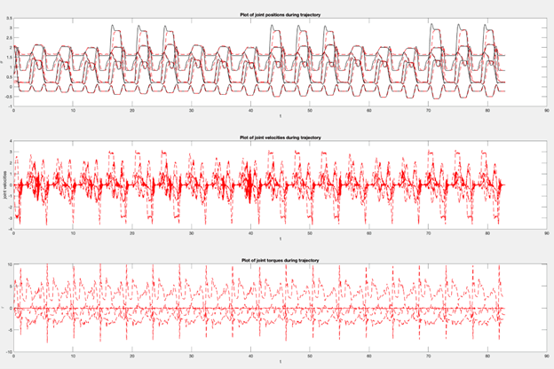
Joint positions, velocities, and torques over time.

• Joint velocities show noise but exhibit periodic patterns matching pick-and-place cycles
• Torques display peaks during 90° rotations for block placement
• Tracking errors indicate room for improved control tuning

Workspace Performance

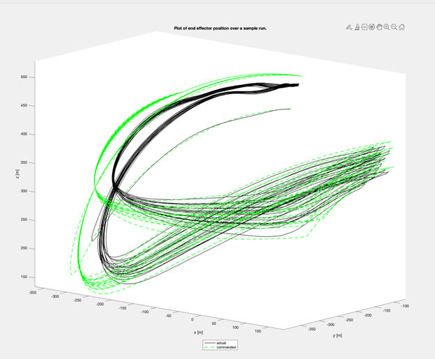
Actual vs. commanded end-effector positions.

Visible deviations between actual and commanded trajectories—particularly in X and Y axes—suggest uncompensated gravity effects. The Z-axis error couples into X/Y motion through the arm's kinematics. A robust gravity compensation scheme or preemptive Z-offset could address this.

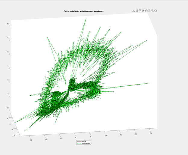
Actual vs. commanded end-effector velocities.

Velocity profiles appear peaky since velocities weren't directly constrained in trajectory generation—they result from position profiles. However, overall velocity tracking follows commanded trends reasonably well.