Hybrid Control for Cable-Suspended Loads with Quadrotors
Multi-agent trajectory optimization with dynamic constraint handling
Project Overview
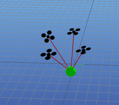
Picture a heavy package being carried by multiple drones, each connected by cables. What happens if one drone fails? The cables go slack, and the system needs to adapt instantly. This project tackles that challenge: how do you plan trajectories when cables can transition between taut and slack? It's a hybrid control problem—the physics changes depending on cable state.
We used trajectory optimization (finding the best path through space and time) with a solver called IPOPT. The key innovation: an active set method that dynamically switches constraints when cables change state. Implementation was done in Julia.
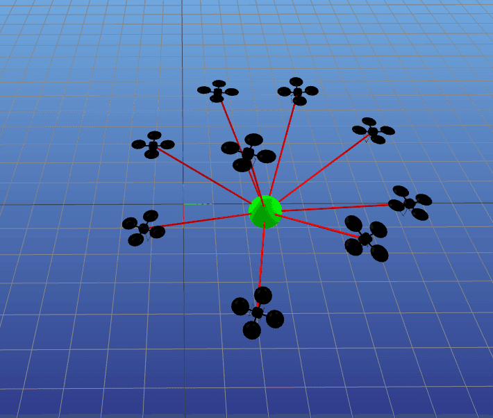
Nine-agent cable-suspended load transport system
Background and Motivation
Using multiple drones to carry loads is attractive: they're flexible, easy to deploy, and can lift more together than alone. But previous work assumed cables always stay tight. In reality, cables go slack—when a drone fails, when there's turbulence, or when maneuvering aggressively. Standard trajectory optimizers like ALTRO struggle with this discontinuity.
Our solution: treat slack as a mode switch. Instead of separate physics models for 'all cables taut' vs 'some cables slack', we use one model with switchable constraints. The optimizer figures out when to enforce cable tension constraints and when to relax them.
Key Innovations
- Active set method for dynamic constraint switching
- Quaternion-based orientation for aggressive maneuvers
- Hybrid state machine for taut/slack cable transitions
- Analysis of
IPOPTperformance in large-scale non-convex problems
Problem Formulation
The math gets involved, but here's the intuition: each quadrotor has 13 states (position, orientation as a quaternion, linear and angular velocity), while the payload is just a point mass (6 states). Cables are modeled as massless rigid links—they transmit force but have no dynamics of their own.
Quadrotor Dynamics
Each drone's motion follows Newton's laws plus the cable force pulling on it:
Quadrotor state dynamics with cable force Fc
Load Dynamics
The payload is modeled as a point mass with 6 states:
Load dynamics with cable forces from L active quadrotors
Optimization Objective
The trajectory optimization minimizes a cost function penalizing state deviation, control effort, and terminal error:
Constraints
- Dynamics constraints — discretized quadrotor and load dynamics
- Boundary conditions — initial and final state requirements
- Cable constraints — fixed length geometric constraint
- Tension constraints — cables can only pull (modified by hybrid logic)
- Motor limits — respecting physical actuator capabilities
- Collision avoidance — safe distances between agents
Hybrid Control Strategy
Here's the heart of the project: the active set method. Think of it as a traffic cop for constraints. When a cable is taut, we enforce that it stays at its fixed length and can only pull (not push). When it goes slack, we drop those constraints—the cable is effectively disconnected. The optimizer solves the trajectory, checks each cable's tension, and updates which constraints are 'active' for the next solve.
1HYBRID CONTROL ALGORITHM
2========================
3
4INITIALIZE:
5  Set all cables to ACTIVE (taut)
6
7OPTIMIZATION LOOP:
8  1. Solve trajectory optimization
9     - Apply full constraints for ACTIVE cables
10     - Apply relaxed constraints for SLACK cables
11
12  2. Evaluate each cable state:
13     IF cable is ACTIVE:
14       IF tension < threshold → set SLACK
15     IF cable is SLACK:
16       IF reattach conditions met → set ACTIVE
17
18  3. IF any state changed:
19       Re-solve with updated constraints
20     ELSE:
21       Apply control, advance to next step
22
23REPEAT until trajectory complete
Julia Implementation
The conceptual Julia code below shows how to define the IPOPT problem for this trajectory optimization:
1using Ipopt
2
3# Problem dimensions
4num_knots = 50
5num_quads = 4
6nx_quad = 13    # states per quadrotor
7nu_quad = 4     # controls per quadrotor
8nx_load = 6     # load states
9
10# Total decision variables
11total_vars = num_knots * (
12    num_quads * (nx_quad + nu_quad) + nx_load
13)
14
15# Objective: tracking error + control effort
16function eval_f(x)
17    cost = 0.0
18    for k = 1:num_knots
19        xq = get_quad_states(x, k)
20        xl = get_load_state(x, k)
21        u  = get_controls(x, k)
22        cost += stage_cost(xq, xl, u)
23    end
24    return cost + terminal_cost(x)
25end
26
27# Constraints: dynamics, cables, bounds
28function eval_g(x, g)
29    idx = 1
30    for k = 1:(num_knots - 1)
31        # Quadrotor dynamics
32        for i = 1:num_quads
33            g[idx] = quad_dynamics(x, k, i)
34            idx += 1
35        end
36
37        # Load dynamics
38        g[idx] = load_dynamics(x, k)
39        idx += 1
40
41        # Cable constraints (hybrid)
42        for i = 1:num_quads
43            g[idx] = cable_length(x, k, i)
44            g[idx+1] = tension(x, k, i)
45            idx += 2
46        end
47    end
48end
49
50# Configure solver
51prob = CreateProblem(total_vars, bounds...)
52AddOption(prob, "mu_strategy", "adaptive")
53AddOption(prob, "tol", 1e-4)
54AddOption(prob, "max_iter", 1000)
55
56# Solve
57prob.x = initial_guess
58status = IpoptSolve(prob)
59solution = prob.x
Hybrid Control Flow
The hybrid control logic is an iterative process: all quadrotors start as active, trajectory optimization is solved, cable tensions are evaluated, state transitions occur as needed (active→slack or slack→active), and constraints are updated accordingly. If any configuration changes, the optimization re-solves with the new constraint set.
Simulation Results and Observations
We tested the framework on configurations from 4 to 9 quadrotors. The good news: IPOPT produces physically reasonable trajectories. The challenge: these problems are highly non-convex (many local minima), and the solver sometimes struggles to find the true optimum. Real-world robotics often means 'good enough' rather than mathematically perfect.
Key Findings
Qualitatively, the trajectories look right—drones spread out, maintain formation, and transport the load smoothly. Quantitatively, numerical convergence was difficult; the solver found feasible solutions but couldn't always reduce constraint violations to machine precision.
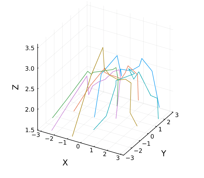
Position plot for a 6-agent configuration from start to goal.
Solver time varied significantly with agent count and problem complexity. Early iterations converged well, but later iterations struggled to reach full convergence.
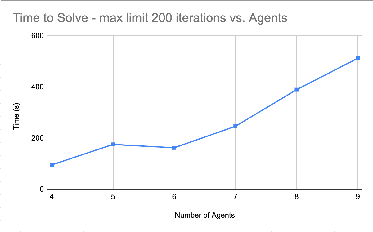
Time required for IPOPT solve for different number of agents.
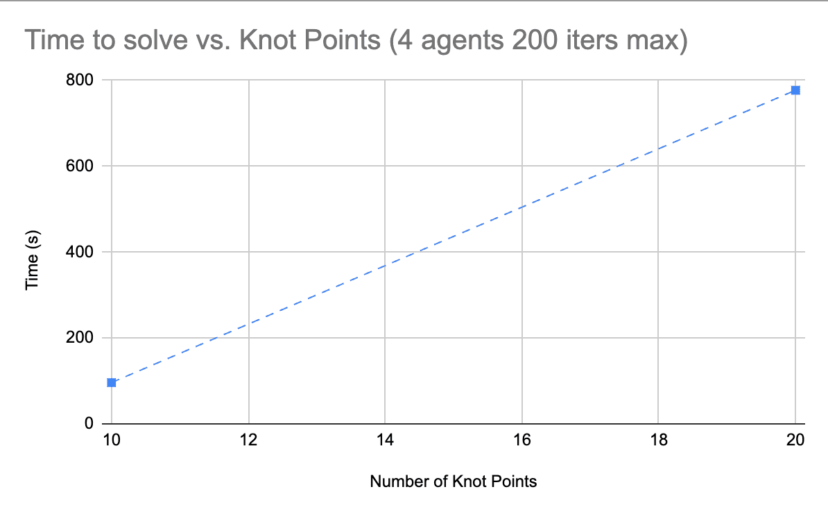
Graph of runtime vs number of knot points.
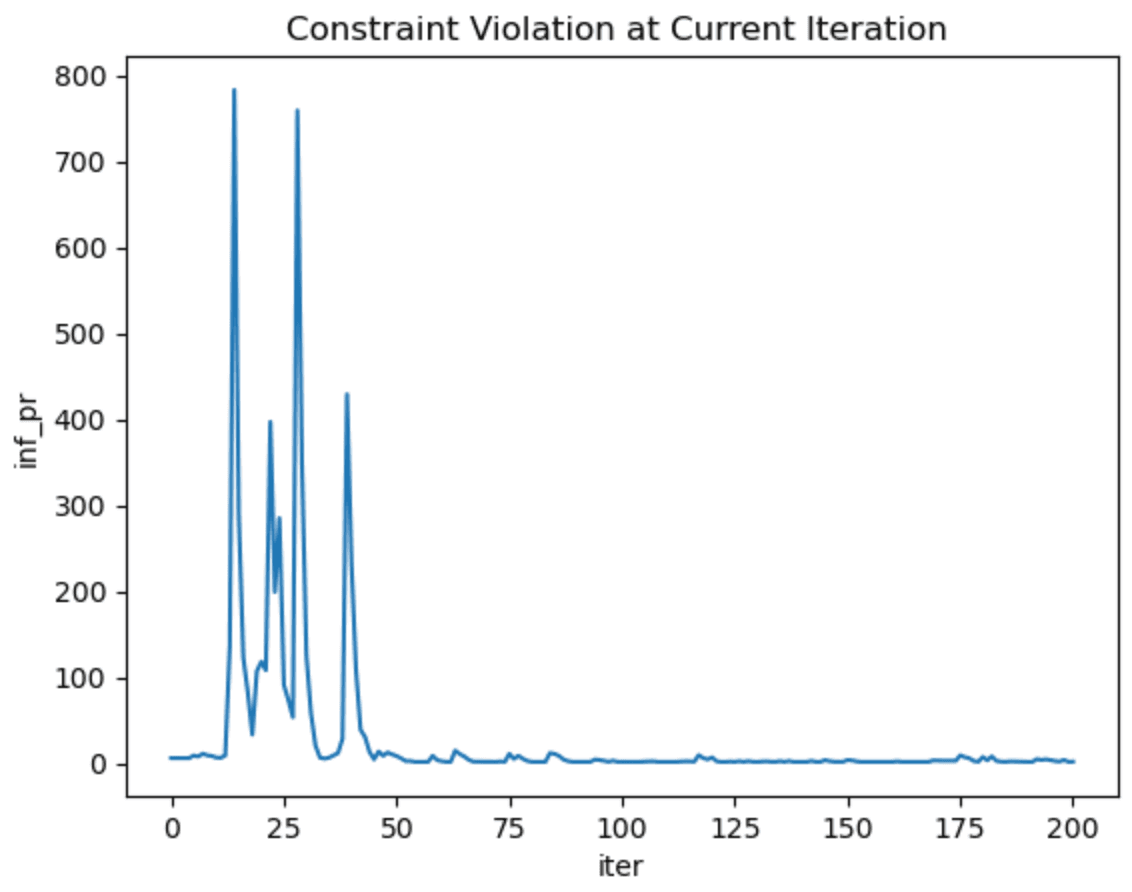
Constraint violations across iterations of IPOPT.
Computational Scaling
Doubling the knot points led to an 8-fold increase in solver time, highlighting the computational complexity. A 100-knot formulation was infeasible—the Jacobian matrix grew to approximately 54 million elements.
IPOPT Limitations and ALTRO as an Alternative
IPOPT is a general-purpose nonlinear optimizer—powerful but not specialized for robotics. ALTRO (Augmented Lagrangian Trajectory Optimizer) is designed specifically for trajectory problems and handles certain challenges better. If I were to continue this work, ALTRO would be the next thing to try.
ALTRO Advantages
- Infeasible initialization — can start from infeasible trajectories (vs. IPOPT needing near-feasible)
- Constraint handling — more numerically stable for obstacle avoidance and state-triggered constraints
- Convergence — less sensitive to initial guess quality
Challenges with IPOPT
Our IPOPT implementation faced convergence challenges due to high dimensionality, non-convexity, numerical instabilities from dynamics/constraints, and sensitivity to initial guesses. These factors make ALTRO a promising alternative for future work.
Conclusion and Future Work
This project shows that cable slack—a real-world problem often ignored—can be handled systematically through hybrid control. The active set method provides a clean way to switch constraints based on physical state. While IPOPT has limitations for these highly non-convex problems, the framework itself is sound and could benefit from better solvers.
Future Directions
- Distributed optimization — reduce problem size and improve scalability
- Distributed slack handling — improve adaptability in dynamic environments
- ALTRO exploration — address initialization and convergence challenges